15 Variant calling
The previous steps of our pipeline were concerned with 1) the quality control of our sequence reads and 2) where all these reads fit on our reference genome. In this final step we will assess the genetic differences between each of our samples and the reference genome. This process is called variant calling or variant detection. While conceptually simple, the main challenge is that it can be difficult to discern sequencing errors from real variants.
The tools and steps involved in the variant calling process are outlined in the diagram below.

Variants can be identified by looking at all the reads at a given position in the genome and looking at the variation present in the different reads covering the position. The more reads that we see that agree on a specific variant compared to the reference genome, the more confident we can be that we are dealing with a real variant, in that particular sample. Of course, there are many considerations to make at this point; we need to take into account the possibility of sequencing errors, mapping errors, the ploidy of our organism, the possibility of complex infections (i.e., multiple genetically distinct parasites in a single sample, instead of a single clone), etc. Moreover, we can compare variants across different samples and perform various filtering steps to reduce the chance of false positives.
We will make use of GATK4 (Genomic Analysis ToolKit) for the variant detection components of our pipeline. This is a very extensive toolkit which offers many different utilities.1
1 GATK is actually a java program, which means that we can pass it additional arguments like memory requirements. See the GATK documentation for more information on this.
15.1 Types of variants
We can identify several different types of genetic variants:
- Single nucleotide polymorphism (SNPs)2
- If a SNP results in an amino acid change, we refer to it as a nonsynonomous substitution (resulting in a &&missense mutation). If there is no change in the amino acid sequence (thanks to codon redundancy), it is referred to as a synonomous substitution.
- If a SNP introduces a stop-codon and results in premature termination of mRNA translation, this is termed a nonsense mutation, if it removes a stop-codon, it is called a nonstop mutation.
- Short insertions and deletions (indels)
- If the indel is not a multiple of three bases, this leads to a frameshift mutation.
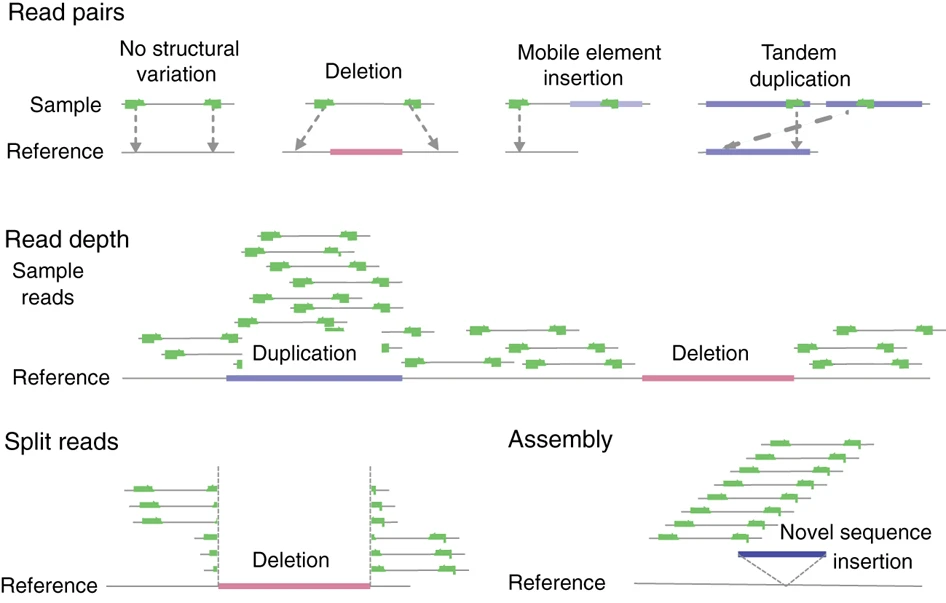
- Structural variants (SVs): larger (chromosomal) rearrangements (> 50 base pairs) like insertions, deletions, inversions, translocations or duplications.
- Copy number variation (CNVs): a particular type of SV caused by the duplication or deletion of a particular DNA segment (e.g., hrp2 and hrp3 genes in P. falciparum).
2 A related term is the single nucleotide variation (SNV). It appears to be more commonly used for somatic rather than germline events, although others use it to describe single nucleotide changes below a certain frequency threshold.
The GATK variant discovery pipeline that we introduce below focuses on short (germline, as opposed to somatic) variants, i.e. SNPs and indels.
Larger structural variant discovery tends to be more challenging than short variant detection. Long-reads help quite a bit, as does paired-end sequencing. Similar considerations apply for calling haplotypes (~ combination of nearby variants, or more strictly: a physical grouping of genetic variants that is inherited together).
Further reading:
15.1.1 Even more indices
Several of the GATK tools require us to index the reference genome again(!), but this time using samtools faidx ref.fasta, resulting in a .fai indexed reference file. Like before, this creates a new file in the reference genome directory, with the extension .fai. Additionally, we also need a .dict dictionary file, which can be created using gatk CreateSequenceDictionary –R ref.fasta.
- Create the two required reference index files for both of your Plasmodium reference genomes.
15.2 Calling (short) variants - GATK HaplotypeCaller
Just like the other steps in our pipeline, there exist many different algorithmic implementations of variant calling, each with their own strengths, weaknesses and intended use cases.
Aside from GATK HaplotypeCaller, you might encounter
- bcftools mpileup (position-based caller, made by the same developers as
samtools) - FreeBayes
We will use the GATK HaplotypeCaller tool to simultaneously detect both SNPs and indels. It uses local de novo assembly of haplotype in regions that show signs of variation. You can find out more about the underlying process in the GATK documentation or in this GATK article.
The tool requires two
gatk HaplotypeCaller \
    -R reference.fasta \
    -I alignment.sort.dup.bam \
    -O output.g.vcf.gz" \
    -ERC GVCF

# optional arguments:
# set number of threads: --native-pair-hmm-threads 2
# set maximum and initial memory usage: --java-options "-Xmx4g -Xms4g"
The output of this process is a GVCF file. It is very similar to the VCF file format, except that it tracks each genomic coordinate instead of only those positions where variations were detected. Also note that the output is compressed with gzip by default.
- Run
gatk HaplotypeCallerfor a single BAM file and inspect the resulting VCF file. - Create your own script to call variants for all for the Peruvian P. falciparum AmpliSeq alignments. Afterwards, compare your approach with the
call_variants.shscript andcall_variants-extended.shscripts.
15.3 VCF files revisited
The output of variant calling is a file in the Variant Call Format (.vcf), which we already encountered in Section 7.1.1.1.

More info can be found on on Dave Tang’s Learning the VCF page
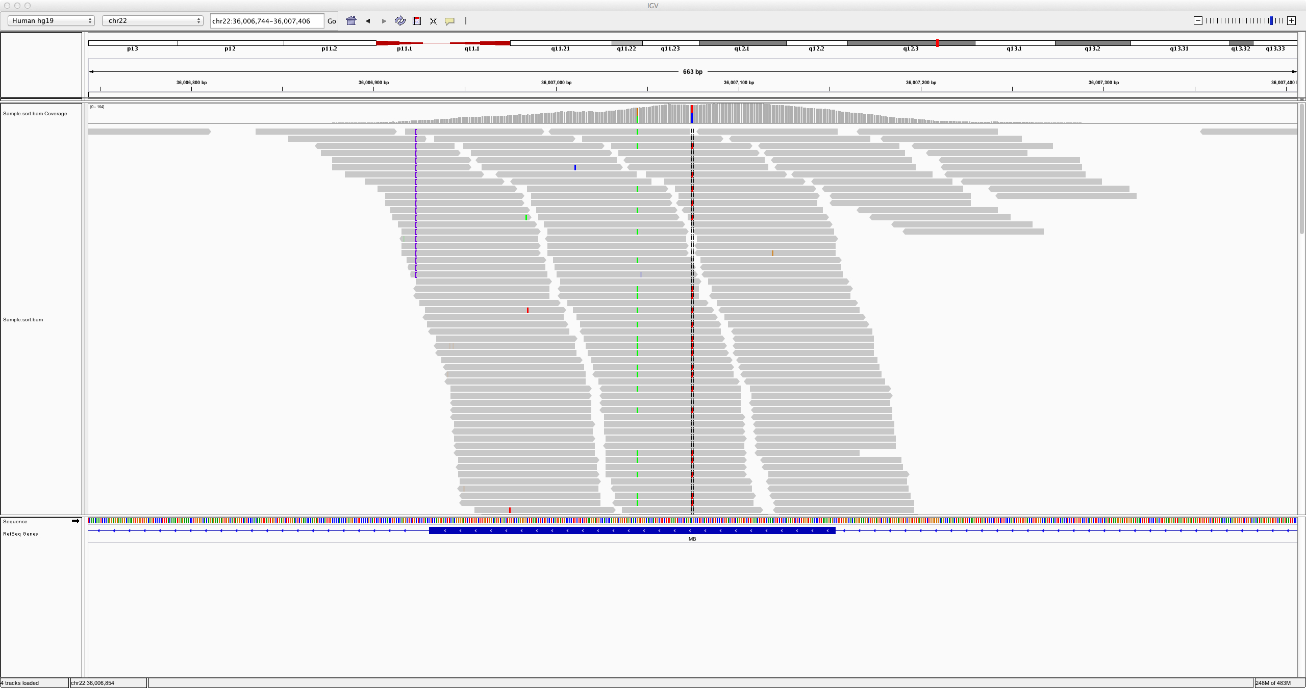
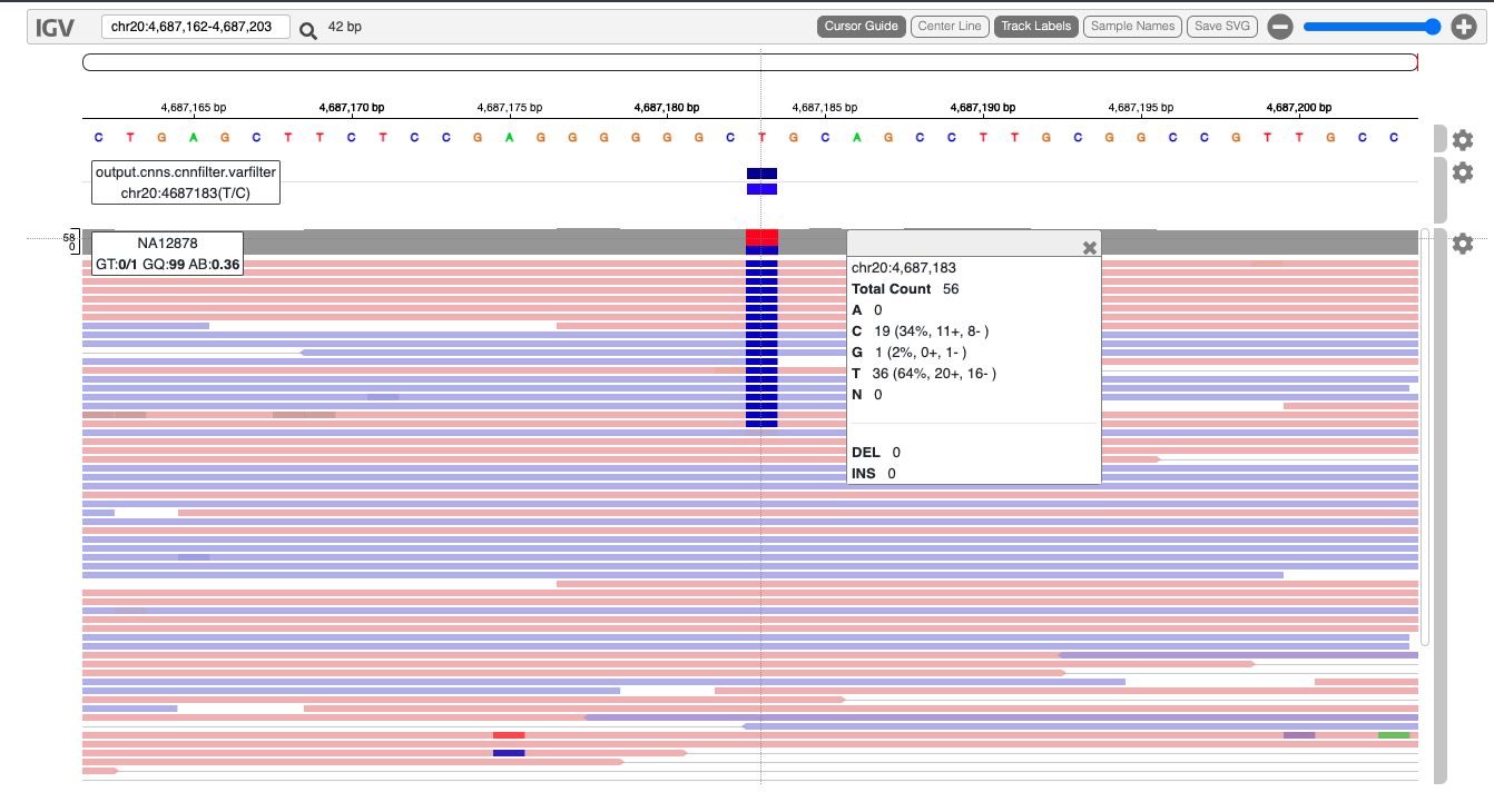
15.4 Visualisation using IGV
Similar to our BAM files, we can visualise VCF files in tools like IGV (Integrative Genomics Viewer). For a tutorial on this, we refer to this Data Carpentry workshop.
15.5 Combine samples
After the previous step, we ended up with a GVCF file for each of our samples. Now we will merge these samples into a single multi-sample GVCF file using either GATK CombineGVCFs (docs) or GATK GenomicsDBImport (docs)3
3 The latter is slightly faster, while the former makes it easier to work with multiple intervals. See this tutorial for an example on how to use CombineGVCFs.
gatk GenomicsDBImport \
    --genomicsdb-workspace-path /path/to/store/database \
    --intervals <genomic-range> \
    --intervals <genomic-range> \
    # ...
    --sample-name-map <cohort.sample_map> \
    --tmp-dir /path/to/large/tmp
# optional arguments:
# set maximum and initial memory usage: --java-options "-Xmx4g -Xms4g"
# number of samples to process simultaneously (affects memory): --batch-size 50
The cohort.sample_map file should contain a list of sample and file names in tab-delimited format:
sample1      sample1.vcf.gz
sample2      sample2.vcf.gz
sample3      sample3.vcf.gz
For a small number of samples, you can also provide each of them directly using multipe -V flags:
gatk GenomicsDBImport \
    -V sample_1.g.vcf.gz \
    -V sample_2.g.vcf.gz \
    -V sample_3.g.vcf.gz \
    --genomicsdb-workspace-path /path/to/store/output/database \
    --tmp-dir=/path/to/large/tmp \
    -L <genomic-interval>
The -L (or --intervals) option is used to define the genomic intervals over which the tool operates. Unfortunately, these intervals need to be prepared and provided manually. For the Plasmodium falciparum Peru AmpliSeq panel, you can use:
Click me to show the full list of intervals:
-L Pf3D7_01_v3:179679-179985 \
-L Pf3D7_01_v3:180375-180467 \
-L Pf3D7_01_v3:190106-191218 \
-L Pf3D7_01_v3:191661-192230 \
-L Pf3D7_01_v3:192264-192925 \
-L Pf3D7_01_v3:192961-194344 \
-L Pf3D7_01_v3:194371-195570 \
-L Pf3D7_01_v3:195762-196800 \
-L Pf3D7_01_v3:196836-200312 \
-L Pf3D7_01_v3:200448-200978 \
-L Pf3D7_01_v3:204949-205193 \
-L Pf3D7_01_v3:339163-339466 \
-L Pf3D7_01_v3:464638-466535 \
-L Pf3D7_01_v3:466803-470193 \
-L Pf3D7_02_v3:519270-519567 \
-L Pf3D7_02_v3:694157-694456 \
-L Pf3D7_03_v3:361017-361320 \
-L Pf3D7_03_v3:849331-849578 \
-L Pf3D7_04_v3:532089-532395 \
-L Pf3D7_04_v3:691941-692036 \
-L Pf3D7_04_v3:747935-749935 \
-L Pf3D7_04_v3:770125-770439 \
-L Pf3D7_05_v3:921740-921999 \
-L Pf3D7_05_v3:957777-958361 \
-L Pf3D7_05_v3:958396-959096 \
-L Pf3D7_05_v3:959153-959988 \
-L Pf3D7_05_v3:960166-961735 \
-L Pf3D7_05_v3:962020-962193 \
-L Pf3D7_05_v3:1188236-1188508 \
-L Pf3D7_05_v3:1214304-1214615 \
-L Pf3D7_06_v3:148637-148858 \
-L Pf3D7_06_v3:635908-636217 \
-L Pf3D7_07_v3:403083-404022 \
-L Pf3D7_07_v3:404296-406440 \
-L Pf3D7_07_v3:455433-455668 \
-L Pf3D7_07_v3:782049-782219 \
-L Pf3D7_08_v3:500969-501114 \
-L Pf3D7_08_v3:548041-549952 \
-L Pf3D7_08_v3:549982-550332 \
-L Pf3D7_08_v3:803010-803329 \
-L Pf3D7_08_v3:1373986-1374244 \
-L Pf3D7_08_v3:1374249-1374474 \
-L Pf3D7_08_v3:1374486-1374705 \
-L Pf3D7_08_v3:1374711-1375419 \
-L Pf3D7_09_v3:230922-231210 \
-L Pf3D7_09_v3:1005112-1005419 \
-L Pf3D7_10_v3:340949-341230 \
-L Pf3D7_10_v3:1172615-1172823 \
-L Pf3D7_11_v3:416182-416488 \
-L Pf3D7_11_v3:874927-875071 \
-L Pf3D7_11_v3:1294408-1295115 \
-L Pf3D7_11_v3:1295124-1295390 \
-L Pf3D7_11_v3:1295423-1295672 \
-L Pf3D7_11_v3:1505334-1505635 \
-L Pf3D7_12_v3:717790-718460 \
-L Pf3D7_12_v3:718476-719820 \
-L Pf3D7_12_v3:1126866-1127122 \
-L Pf3D7_12_v3:1552012-1552292 \
-L Pf3D7_12_v3:1611167-1611448 \
-L Pf3D7_12_v3:2091976-2094267 \
-L Pf3D7_13_v3:1595960-1596123 \
-L Pf3D7_13_v3:1724599-1727164 \
-L Pf3D7_13_v3:1827453-1827763 \
-L Pf3D7_13_v3:2503123-2503359 \
-L Pf3D7_13_v3:2503390-2505580 \
-L Pf3D7_13_v3:2840639-2841793 \
-L Pf3D7_14_v3:293359-293982 \
-L Pf3D7_14_v3:294267-294832 \
-L Pf3D7_14_v3:832462-832742 \
-L Pf3D7_14_v3:1381895-1381990 \
-L Pf3D7_API_v3:24048-34146 \
-L Pf_M76611:3384-4634
For the other AmpliSeq panels, check out the pipelines by Eline Kattenberg on GitHub.
For whole-genome sequencing, the MalariaGEN Pf7 database uses 10 kilobase intervals (and -ip/--interval-padding 500 to add some padding) (see methods).
Merging GVCF files can be quite slow. GATK has written an article on how to address performance issues.
Merge the GVCFs for all Peruvian Plasmodium falciparum AmpliSeq samples.
15.6 Joint genotyping
After combining the GVCF files for all our samples, it is time to perform joint genotyping using GATK GenotypeGVCFs (docs). The main idea behind this step is to improve the inference of variant detection by leveraging the information that is present across all samples in our cohort. For more information on the logic behind joint genotyping, we refer to this GATK article.
gatk GenotypeGVCFs \
    -R reference.fasta \
    -V gendb://genomicsDB \
    -O variants.vcf.gz \
    --tmp-dir /path/to/large/tmp

# optional arguments:
# set maximum and initial memory usage: --java-options "-Xmx4g -Xms4g"- Perform joint-genotyping for the multi-sample VCF file with the Peruvian Plasmodium falciparum AmpliSeq samples.
- Inspect and visualise the output VCF (optionally using IGV).
Have a look at GATK’s article on VCF files, in particular the section on the structure of variant call records and how to interpret them: https://gatk.broadinstitute.org/hc/en-us/articles/360035531692-VCF-Variant-Call-Format.
15.7 Variant filtering
Not all the variants present in our VCF file are likely to be real. Therefor, a final step in our pipeline is to filter out variants that are likely to be errors. We will discuss two different approaches: Variant Quality Score Recalibration (VQSR) (recommended by GATK) and hard-filtering.
Hard-filtering works by setting specific thresholds for one or multiple annotations (i.e. properties of a variant, like read coverage, proportion of forward/reverse reads, etc.) VQSR is a more powerful because it tries to combine all of these annotations to make a decision about good or bad variants, but to do this, it require a large number of samples and a database of well-curated known variants. Therefor, we do not recommend it for AmpliSeq data, but it is probably a good idea to use it for WGS data.
The GATK tool that performs hard-filtering is GATK VariantFiltration (docs). The two main options are --filter-name and --filter-expression, which allow you to set a particular threshold for an annotation. For example, the code below filters out variants which have a sequencing depth lower than 10 (DP < 100):
gatk --java-options "-Xmx7g" VariantFiltration \
    -R reference.fasta \
    -V variants.vcf.gz \
    -O variants.filter.vcf.gz \
    --filter-name "DP100" \
    --filter-expression "DP < 100"
Running the above will create a VCF file where the filter column is said to PASS or not depending on the filters that were applied. In order to actually remove the suspected bad variants from the file, we still need to run the following:
gatk/gatk SelectVariants \
    -R reference.fasta \
    -V variants.filter.vcf.gz \
    --exclude-filtered \
    -O variants.filter.pass.vcf.gz

# or equivalently
bcftools view -f 'PASS' -O vcf -o variants.filter.pass.vcf variants.filter.vcfThe filtering steps should ideally be performed separately for both SNPs and indels. You can split your VCF file via:
# create SNPs-only subset
gatk SelectVariants \
    -V cohort.vcf.gz \
    -select-type SNP \
    -O snps.vcf.gz

# create indels-only subset
gatk SelectVariants \
    -V cohort.vcf.gz \
    -select-type INDEL \
    -O indels.vcf.gz
    --select-type mixed
After filtering, they can be merged back together.
See here (section 2) for more info on the --select-type flag.
- For hard-filtering AmpliSeq data, you can explore the P. falciparum AmpliSeq Peru pipeline.
Further reading:
- Overview of annotations to filter on: https://gatk.broadinstitute.org/hc/en-us/articles/360035890471-Hard-filtering-germline-short-variants
- Hands-on GATK filtering approaches: https://gatk.broadinstitute.org/hc/en-us/articles/360035531112–How-to-Filter-variants-either-with-VQSR-or-by-hard-filtering
- https://www.melbournebioinformatics.org.au/tutorials/tutorials/variant_calling_gatk1/variant_calling_gatk1/#section-4-filter-and-prepare-analysis-ready-variants
- https://speciationgenomics.github.io/filtering_vcfs/
- https://sib-swiss.github.io/NGS-variants-training/2021.9/day2/filtering_evaluation/
- https://qcb.ucla.edu/wp-content/uploads/sites/14/2016/03/IntroductiontoVariantCallsetEvaluationandFilteringTutorialAppendix-LA2016.pdf
- https://app.terra.bio/#workspaces/help-gatk/GATKTutorials-Germline
15.8 Annotation of variants
The final step in our pipeline is to annotate variants. For this, a tool like snpEff can be used. You can see it being used in the AmpliSeq pipeline here.