13  Quality control and trimming

The first step in our pipeline deals with assessing the quality of our sequence reads and when necessary cleaning them. The reads are provided to us by the sequencer in the form of FASTQ (or fastq) files. We already introduced this file format in a previous chapter (Section 5.1.3.1), but we will dive in a bit deeper this time around.

13.1 FASTQ file format revisited

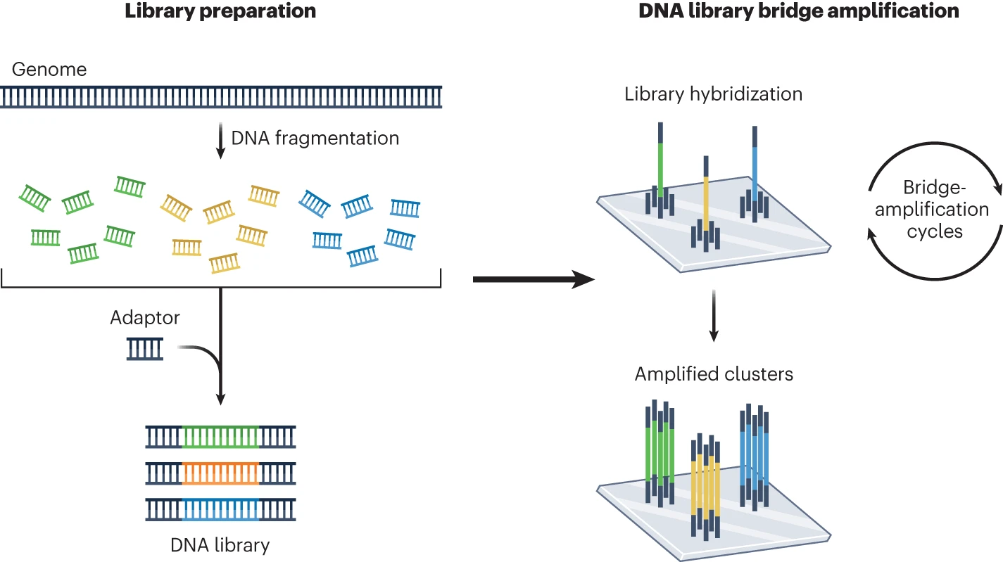
The FASTQ file format holds the raw sequencing reads generated by next-generation sequencing technologies. For the Illumina platform, they contain the sequence data from the clusters on the flow cell (after some initial filtering steps) and these are the types of files that you would receive after a sequencing run. FASTQ files look superficially similar to FASTA files, in the sense that they hold sequence of nucleotides (strings of ACTG characters) preceded by an identifying header (> ...), but they also contain additional information that encodes the base quality scores.

FASTQ files and Illumina sequencing

A more in-depth explanation on FASTQ files can be found on the Illumina website.

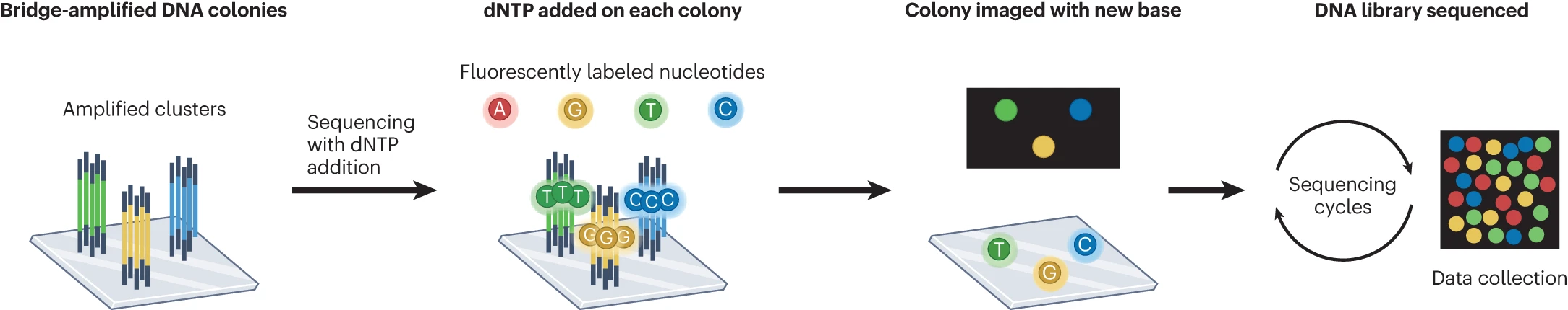
If you need a refresh on the Illumina sequencing technology, i.e. cluster generation on flow cells and sequencing-by-synthesis, you can also check out the following resources:

• Short video by ClevaLab (ClevaLab 2022b) - also available as a blog post (ClevaLab 2022a)
• Next-Generation Sequencing Glossary on the Illumina website (n.d.)
  • this glossary is especially helpful to brush up on terms like cluster, insert, adapters and multiplexing.
• In-Depth NGS Introduction by Illumina (2017)
• Longer video on Illumina platforms (40 min) by Illumina (2021a)
• Reviews on NGS technologies:
  • DNA sequencing at 40: past, present and future (Shendure et al. 2017)
  • The chemistry of next-generation sequencing (Rodriguez and Krishnan 2023)
• Excellent blogpost by Loren Launen (accompanying video lectures are available too) (Launen 2017)
• Short course on MiSeq system by Illumina (focus on imaging and base calling)

---

Library preparation and bridge amplification on flow cell.

Sequencing-by-synthesis and fluorophore imaging or base calling.

Figure 13.1: Overview of Illumina sequencing chemistry (Source: Rodriguez and Krishnan 2023).

FASTQ files are plain-text files consisting of the following four lines for each sequence read:

Line	Description
1	Identifier or header: always starts with ‘@’ and contains information about the read (free format)
2	The sequence of nucleotides making up the read
3	Always begins with a ‘+’ and sometimes repeats the identifier
4	Contains a string of ASCII characters that represent the quality score for each base (i.e., it has the exact same length as line 2)

FASTQ files generally contain many sequences, each of which might look something like this:

@M05795:43:000000000-CFLMP:1:1101:21302:1790 1:N:0:44
CCTCACCATGCAACCGATGCTCATCATGCAGCCGATGCTCATCATTCTCATCATGCACCCGCTGTCTCTTTTACACTTCTCCTTTCCCACGTCTCCCTTCTTTTTCTCCTATCCCTTCTTCTTCTTTCCCTCTTTTTTCTTTTTTCTTTTTCTCTTTTTTTCTTTTTTTCCCCTTTCTCTCTCTCTTTTCCTCTTCTTCTTCTTCTCTTCCTTCCCCCCCCCTTCCCTCTCCCCTCTCTCTTCCTCTTTCCCCCTTCTTTCCTTCCCCCCTCCCCCTTCCCTCCCCTTTCATCTCTTCCT
+
-AACCFGGGGGGGGFEGGCFGGCCFGGGGGGFDCCFGGEF9FA9F,6;C,CC,E,6,,;,++6+B6,<CE,6,6,9,95,,5,,,,,5,4+,,,,,9,,,,,5,5,9,,9,9,45,944,,5,4,9,,,,,,,,,,,+,,,,,,+,,,,,,,,,,,,,,++,,3,,,++,,,,,,,,,,,+++++++++++++1+++++++++++++++++++0****/())()/(()()(((((((())))))))))))))((((,))))))-),(((((((,((((((()(((((())-)-)))))))

The header line always starts with an @ and usually carries information on the sequencing run, cluster on the flow cell or any other metadata. Note however that this format is not entirely fixed and depending on how and where your sequences were generated, the headers might look slightly different. In this case, the read was sequenced on an Illumina 1.8 sequencer, and we can identify the following types of metadata, separated by colons : and forward slashes / as field separators:

@<instrument>:<run number>:<flowcell ID>:<lane>:<tile>:<x-pos>:<y-pos> <read>:<is filtered>:<control number>:<barcode sequence>

• @: start of the header
• M05795: unique sequencing instrument ID
• 43: run number
• 000000000-CFLMP: unique flow cell ID
• 1: lane number (see below for more info on lanes)
• 1101: tile number (= section of the lane)
• 21302: x-coordinate of the cluster
• 1790: y-coordinate of the cluster
• 1: read number - 1 or 2 for paired-end sequencing
• N: not filtered
• 0: control number
• 44: index/barcode sequence (see below for more info on barcoding and multiplexing)

The second line contains the sequence as a string of characters. The third line is basically a historical artifact that we’re now stuck with. The fourth line, containing the quality scores, will be explore in more detail in the next section (Section 13.2).

---

FASTQ files are typically named using the following convention:

SampleName_S1_L001_R1_001.fastq.gz

where:

• SampleName is the name of the sample as it was provided in the samplesheet during submission, or a unique sample ID otherwise.
• S1 is the sample number, again based on the samplesheet.
• L001 is the lane number on the flow cell.
• R1 is the read pair - 1 or 2 for paired-end sequencing (or I1/I2 for index reads).
• 001is always the last part of the name.

Putting it all together, we end up with:

{sample_name}_S{sample number}_L{lane number}_{R/I}{read or index number}_001.fastq.gz

Warning

Keep in mind that these are conventions, not strict rules, so you will likely encounter file names that differ from the above.

Similar caveats apply to the header lines inside FASTQ files.

Also, note that there is no standard file extension for FASTQ files, both .fq and .fastq are common. Keep in mind that file extensions in general are arbitrary; it is the file content that determines the file format, not the extension (although both Windows and Mac might try to convince you otherwise). However, using standard and descriptive file extensions makes everyone’s life much easier.

---

FASTQ files can typically contain up to millions of reads (depending on the depth of sequencing), resulting in file sizes in the range of hundreds of MBs to multiple GBs. However, the files are usually compressed using gzip (receiving the .fastq.gz extension) to reduce their file size.

Compress your files!

Throughout this pipeline (and in many other bioinformatics analyses) you should avoid using and storing uncompressed files, because they waste disk space. Moreover, many of the formats we will talk about are also faster to analyse in binary compressed form compared to the plain-text versions (e.g., BAM vs SAM, see Section 6.2.1 and Section 6.4.1).

Refer to Section 6.4 or this overview for a refresher on file compression.

The raw FASTQ files forms the basis on which your analysis builds. No matter what analysis you might perform, you should be able to reproduce it if you can start from the same raw reads. It is therefor of utmost importance to properly manage these files and store them in a secure location, preferably backed up.

---

A sequencing run will generally produce either a single FASTQ file per sample (for single-end runs) or a pair of files per sample (for paired-end sequencing). For the latter, the files will bear identical file names, except for the suffix to distinguish them easily (and programmatically), usually either _1/_2 or R1/R2. E.g., the two files might be called SampleName_S1_L001_R1_001.fastq and SampleName_S1_L001_R1_001.fastq. In some circumstances you might end up with a third file (either without a suffix or tagged as _3), e.g., containg unpaired reads.

Tip 13.1: Paired-end sequencing

In a nutshell: in paired-end sequencing, both ends of the DNA fragments in the library are sequenced inwards (5'-F===>_______<===R-3') one after the other (the Forward and Reverse read).

The forward and the reverse reads do not necessarily overlap; this depends on the length of the insert and the number of sequencing cycles used for each round of sequencing. Indeed, in many cases the forward and reverse reads are a couple of hundred bases apart, pointing towards each other, because the DNA insert is longer (e.g., ~300 bp) than the forward or reverse read (e.g., 150 bp each, including read primers). So to emphasize, we do not expect the forward and reverse reads to cover identical sections of the fragment.

What is the point of paired-end sequencing? Well, because we know what the average distance between the forward and reverse read is ¹, alignment algorithms can make use this information to more accurately map the reads across repetitive regions in the genome (see Figure 13.2), which would otherwise be even more problematic.

Figure 13.2: Paired-end sequencing and alignment. (Source: Illumina 2017)

These paired reads are usually results in two separate files; read 1 and read 2 R1/R2 (not to be confused with mate-pairs).

The forward and reverse read pairs are split across these two files and they always appear in the same order (or at least this is what most downstream tools expect).

¹ During library construction, we target a specific size distribution or range of DNA inserts, either through the fragmentation process, or in the case of AmpliSeq, by directly generating amplicons of known specific sizes.

Inspect the first lines of two paired FASTQ files

• Can you tell by the headers that the sequences are paired and appear in the same order?
• Check the sequence length of each pair and explain why they are (not) the same based on the sequencing process.
• Do the sequences appear to overlap?

You can find paired FASTQ files in the data directory of the training environment.

Solutions

The following bash snippets prints the first reads from two paired FASTQ files:

# print the first 4 lines (= 1 read) of read 1 and read 2 to the console
for fq in ./data/fastq/PF0097_S43_L001_R*_001.fastq.gz; do
    echo "Read ${fq}"
    zcat ${fq} | head -n4
    echo
done

# note that a command like the one below will not work! Why?
zcat training/data/fastq/PF0097_S43_L001_R*_001.fastq.gz | head

Output:

Read ./data/fastq/PF0097_S43_L001_R1_001.fastq.gz
@M05795:43:000000000-CFLMP:1:1101:15977:1738 1:N:0:43
CACAATCAATATCATTATTATTTTTTTTTTTTTTTTTTTTTTTTTTTTTTCTTTTTTTTTCTTTTTCCTTTTTTCTTTTTTTCTTTTTTTCTTTTCCTTTTTTTTTTTCTTTTTCCAATTTATTTTTTTTTTTTTTTTTTTTTTTATTCTTTTTTTTTTCCTTTTTTTTTTTTTTCTTATTTTTTTTTACTTCTTTCTATATTTTATTTCCTTTTCCTCTTTTCCTTTTTCCAATTTTTTTTTCCCCTTTTCCTTTTCCCCTTTTCCTTATTCCTTCATTTTTTTTTTTACCTCCCACCT
+
A8BCCGGFFGFGGCGGFFG<FGGGGGGGGGGD77+@7+@::CC+=@+@:+,<,<A97+++,8<5<,3,,3,:=7,,3E9,++,,3388:1,,3@;,,,33?DBC77**,,,7<,2,,,,7,,,,,,,::>C?5**/5*8:C558**++++0+<<CEEE88+++3<<5*:5:?CE5+++++*2*2975)******84********************/**)**)*.)).49())))-.64((-4())(.48)).)6:7--)(,.4)-).)))-)).))))))))--3(((()))),(2(((

Read ./data/fastq/PF0097_S43_L001_R2_001.fastq.gz
@M05795:43:000000000-CFLMP:1:1101:15977:1738 2:N:0:43
CATACTTTTGTTTATTTTCCTCTTCTTCTTTTTCTTGTTATTTCTTCTTTTTAATATTTACTTCTTACTTTTTCTTTTTTTGTTTACGTTTCATTTTATTTTCTTATACTATCTATATATATTCTATTTTTTAATTATTTTACAATCTTTATGACAAACATAATATTTTATATAAATATGATTTATACTATACTCTCAACATATATTCCTTTGCCCAGCGCTATCAAAAATGCAAATGACAATCTGTCTAAAGTAAATATGGATAACGATATAAATCTTAATAATCACCATAATATAAAAA
+
-,,,8=66@,;,,,=,,666C<CE,,<,<,6C,,;,,6;,;,,,,<,<,<6,,,,,,66,,;,,,,,,,,,,,,;,5,,+++,,,,,,,,,,,:A,,,,,,94,,,9,,9,,,9,9,,,9,9;DD,C;===8,,9,,934=94,,91@=A,9,,++++6+6++++3++++++++++2*?**4+4+0****2*5;DDD**)*0***33;*000***))))0)158)****)1*****0**9***)**002***52*0*3*2*6*:***1)0)1*2*27:A*****2**0)*:*5*9?5*5**

We can see that the header of the first sequence in each FASTQ file is identical, except for the 1/2 near the end, indicating that the reads are derived from the forward and reverse pass of the same cluster on the flow cell.

The two sequences are exactly the same length, and this is what we expect in most cases when the forward sequencing cycle has the same length as the reverse one. Looking ahead at Figure 13.3, we know that the library fragment is sequenced from both ends, for a fixed amount of cycles (in this case, 300 bp).

Depending on the size of the insert, there may or may not be overlap between the two sequences. To be certain, one of the reads will need to be reverse complemented (because they were synthesised based on complementary template strands). In this case, there does not appear to be any. We could check later to see which amplicon this sequence aligns to; if it is longer than 600 bp (= twice the length of each 300 bp fragment), we would not expect to see any overlap.

Below is a code snippet that takes the reverse complement, but you could use an online converter too.

zcat ./data/fastq/PF0097_S43_L001_R2_001.fastq.gz | head -n4 | seqkit seq --seq-type dna --reverse --complement
[INFO] when flag -t (--seq-type) given, flag -v (--validate-seq) is automatically switched on
@M05795:43:000000000-CFLMP:1:1101:15977:1738 2:N:0:43
TTTTTATATTATGGTGATTATTAAGATTTATATCGTTATCCATATTTACTTTAGACAGATTGTCATTTGCATTTTTGATAGCGCTGGGCAAAGGAATATATGTTGAGAGTATAGTATAAATCATATTTATATAAAATATTATGTTTGTCATAAAGATTGTAAAATAATTAAAAAATAGAATATATATAGATAGTATAAGAAAATAAAATGAAACGTAAACAAAAAAAGAAAAAGTAAGAAGTAAATATTAAAAAGAAGAAATAACAAGAAAAAGAAGAAGAGGAAAATAAACAAAAGTATG
+
**5*5?9*5*:*)0**2*****A:72*2*1)0)1***:*6*2*3*0*25***200**)***9**0*****1)****)851)0))))***000*;33***0*)**DDD;5*2****0+4+4**?*2++++++++++3++++6+6++++,,9,A=@19,,49=439,,9,,8===;C,DD;9,9,,,9,9,,,9,,9,,,49,,,,,,A:,,,,,,,,,,,+++,,5,;,,,,,,,,,,,,;,,66,,,,,,6<,<,<,,,,;,;6,,;,,C6,<,<,,EC<C666,,=,,,;,@66=8,,,-

---

For deep sequencing, you might receive multiple files for each sample split across different lanes of the sequencer, in which case you might see files such as SampleName_S1_L001_R1_001.fastq.gz, SampleName_S1_L002_R1_001.fastq.gz. The lane descriptor is also important in the case of multiplexed samples (see Section 13.1.1).

13.1.1 Multiplexed samples

It is often beneficial to pool samples from multiple individuals or projects together and then sequence them in a single run. It saves on costs, makes more efficient use of reagents and it also helps guard against batch effects. This last part is explained by the fact that every sequencing run, and even all the different lanes of a single run, will introduce some technical variation into your experiment. By pooling samples and loading them in the same lane of a single run (or across multiple lanes if more sequencing depth is required), this batch effect or bias can be reduced. When targeting specific genomic areas, like we do for AmpliSeq, or when working with small genomes in general, pooling also allows us to analyse a large amount samples in a single run.

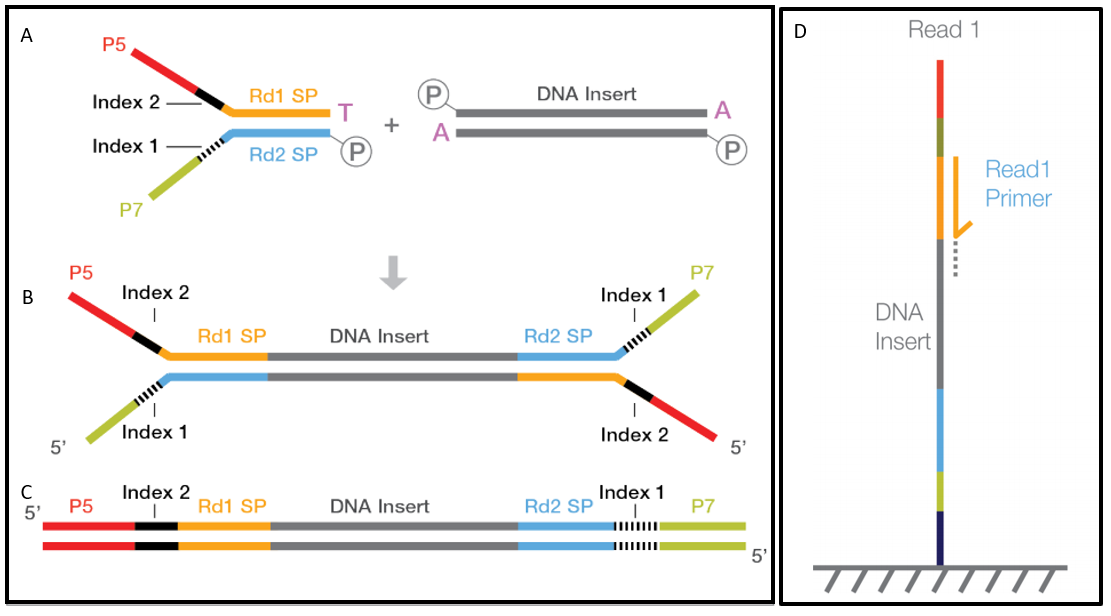
However, if we were to just throw together the DNA from all those different samples and load this mixture onto the sequencer, we would not be able to tell which reads came from which sample afterwards. In order to be able to distinguish reads from different samples, the library fragments need to be tagged with an index (or barcode, naming conventions are messy ²) that is unique to each sample, prior to pooling. During sequencing, the indices of each cluster are read out (in a separate reaction³ from the target DNA of interest, referred to as the insert), and afterwards this information is used to disentangle the different samples and generate (pairs of) FASTQ files per sample.

² in practice, the terms index and barcodes are often used interchangeable for Illumina sequencing, see Illumina (2017). However, sometimes two different types of indices are defined. 1) Multiplex indices are the ones shown in Figure 13.3 which are used for associating reads with samples. They are positioned outside of the insert and have their own sequencing primer (i.e. they are read out during a separate sequencing step and do not show up (at the start) of the FASTQ reads). 2) Inline indices on the other are part of the DNA insert and are read out during the same sequencing step as the DNA insert. Consequently, these do show up in the FASTQ reads and they take up some of the available read length (i.e., the read length available for sequencing of the actual insert is reduced by the length of the inline index). Lastly, the term barcode is also used in other sequencing technologies, like 10X single-cell sequencing, where they are used to uniquely identify beads (~ single cells), rather than multiplexed samples. For Illumina sequencing, a related approach is that of unique molecular identifiers (UMIs), which label each each molecule in a sample in order to reduce the impact of PCR duplicates and sequencing errors.

³ Sequencing the index in a separate step avoids issues with base calling quality degradation, avoids consuming part of the read length available for the insert, and ensures that the index sequence is always complete.

The demultiplexing step is usually handled by the sequencer itself, so the FASTQ files that we end up with are already cleaned and representing a single sample-lane combination.

The index is a unique oligonucleotide sequence that is read separately from the target DNA of interest (called the insert). Depending on the technology, there might even be dual indices ⁴ (on both the 5’ and 3’ ends), placed between the insert (and its sequencing primers) and the adapters (P5/P7, used to anneal the entire DNA fragment to the flow cell) (Figure 13.3).

⁴ sometimes dual indices (UDIs) are used on either end of the library fragment, instead of a single index. See https://knowledge.illumina.com/library-preparation/general/library-preparation-general-reference_material-list/000002344]).

Figure 13.3: Construction of a sequencing library fragment through adapter ligation: P5 (red) / P7 (green) = sequences for anchoring to flow cell; (Rd1 SP (orange) / Rd2 SP (blue) = read 1/2 sequencing primer; index/barcode 1/2 = sample identifiers for multiplexing (Source: Illumina 2020).

• (More information on the molecular technologies used for indexing can be found in Illumina 2021b.)
• (More information on multiplexing and the different sequencing read steps involved can be found in Illumina 2008.)

13.2 Quality control (QC)

As mentioned above, FASTQ files contain information about:

• the raw sequence of base calls
• the quality scores (per base!)
• the location of the cluster on the flow cell
• indirect information on the overall nucleotide composition
• indirect information on the location of the base in the sequence

These different types of data can all be used during the QC of the reads.

13.2.1 Sources of errors

In Illumina sequencing, sequences reads are constructed by detecting the nucleotides present in each particular cluster ( = group of identical elongated fragments) on a flow cell through a fluorescent signal. The intensity and purity of this signal is used to measure the quality of a particular base call, or in other words, how confident we can be that the base call at a particular position in the read is accurate.

Accurately inferring which type of nucleotide got incorporated by each fragment making up a single cluster, for all the millions of clusters on a tiny flow cell simultaneously, for hundreds of cycles in a row, is no easy feat. And as with all (sequencing) technologies, there are a few technical limitations. It is these issues inherent to the sequencing-by-synthesis process that can result in quality degradation, but poor quality scores could also be indicative of more serious problems during the sequencing process or sample preparation.

Some examples of problems that can occur are (University of Exeter DNA sequencing service; Piper et al. 2022; Ledergerber and Dessimoz 2011):

• Signal decay due to degrading fluorophores and some strands in a cluster not being elongated; quality is reduced with each successive cycle (expected, technology limitation).
• Frequency cross-talk caused by frequency overlap of the fluorophores (expected, technology limitation).
• Phasing and pre-phasing: signal noise or ambiguity introduced by lag between the different strands in a cluster. I.e., individual strands fall out of sync, blurring and reducing the true base signal over the remainder of the run.⁵ This problem typically occurs towards the ends of the reads and results in poorer quality with each successive cycle (expected, technology limitation).
• Low complexity sequences (= high AT- or GC-content). A well-balanced nucleotide diversity is required to accurately identify the location of clusters.
• Over-clustering leads to signals from adjacent clusters bleeding through one another. Choosing an optimal cluster-density is the best way to avoid this.
• Instrument breakdown: usually an obvious and sudden drop in quality across many reads. In these cases re-sequencing by the sequencing facility might be required.

⁵ Phasing can be caused by the 3’ terminators not being removed from some fragments in a cluster, in between sequencing cycles. Pre-phasing can happen when two nucleotides get incorporated in one cycle, instead of a single one (e.g., because the 3’ terminators were not effective).

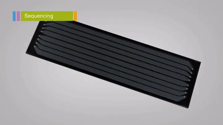
For non-patterned flow cells⁶, there can be close to a million clusters per square millimeter! No wonder the machine can have trouble distinguishing the signal from each of those.

⁶ Newer Illumina instruments use patterned flow cells, where clusters are created inside nanowells at fixed locations on the slide.

Fluorescent signals from clusters on flow cell (Source: Illumina 2016).

13.2.2 Quality scores

The fourth line of each sequence in a FASTQ file contains the so called Phred Quality Scores Q. This line consists of a string of characters, one for each base in the sequence, that encodes the score for that base. The higher the score, the higher the probability that the base was called correctly (or the lower the probability of a misidentification). Specifically, the score is defined as follows:

Q_{PHRED} = -10 \times \log_{10}(P_e)

Where P_e is the probability of an incorrect base call. The following table gives an indication of how to interpret various ranges of quality scores:

Phred Quality Score	Probability of incorrect base call	Base call accuracy
10	1 in 10	90%
20	1 in 100	99%
30	1 in 1000	99.9%
40	1 in 10,000	99.99%
50	1 in 100,000	99.999%
60	1 in 1,000,000	99.9999%

In general, Q30 is considered a good benchmark for reliable base calls.

However, when you look at what is actually in the fourth line of a read in a FASTQ file you will see a rather strange collection of characters, including letters, numbers and other symbols, instead of, well, human-readable scores. What does a score of @ even mean? Well, these are ASCII characters and they are used to compress the Q scores (which are often 2 digit numbers) down into a single character. This not only saves space, but allows the score to be aligned with its corresponding base in the sequence.

The characters in the ASCII set are tied to a particular Q score, but rather than starting from 0 (the first character in the ASCII set), each sequencing platform uses a particular off-set, i.e. they start at a unique base value and count up from there. For example, the current standard for Illumina platforms (1.8) is the Phred+33 encoding, in which a score of 0 corresponds to the character ! and higher scores step through the range of characters from there. The Phred+33 encoding is visualised in green in Figure 13.4.

Figure 13.4: FASTQ quality scoring and ASCII offsets. (Source: Batut et al.; Hiltemann et al. 2023)

Interpreting Phred Quality Scores - example calculation

Consider the following Illumina 1.8 read:

@SR.1:Pf3D7_01_v3:M:533192-533407
TCTCATCATCCCTCTCATCATCATCATCACTCTCATCATTATCATCACTCTCATCACTCTCATTACTATCATCACTCTCATCATTATCATTACTATCATC
+
CABDAAFCBAHCEGFFA?FEEAFFHDCFCB?GHDECDCABFGBGA@HDGGEAABCDA@I?IIDIIH85:=;<:;;97:78:881//-23200&')$'(#%

The first base in the sequence (T) is associated with the encoded Q score C. In Figure 13.5, you can see that the value of this ASCII character is 67.

If we subtract the off-set, we get 67 - 33 = 34, which is the Q score.

Lastly, we need to rearrange the quality score equation shown above and plug in Q in order to obtain the probability of an incorrect base call:

P = 10^{\frac{Q}{-10}} = 10^{\frac{34}{-10}} \approx 0.0004

Or a 0.9999% base call accuracy.

Figure 13.5: ASCII table

To summarize, Q scores can be converted into the probability of base calling errors by performing the following steps:

1. Find the value of the ASCII character.
2. Convert into a Q score by subtracting the off-set value (e.g., -33).
3. Plug the resulting value into the formula P = 10^{\frac{Q}{-10}} to obtain the error probability.

Exercises

Given the following read from a sequencer using the current Illumina 1.8 Sanger+33 format.

@M00984:14:000000000-AA0HF:1:1101:23031:1298 1:N:0:1
CGTGCCAACGGCACTCGTACACGAGTTGTACAGAAACTGAT
+
CCCCCGGGGGGGGGGGGGGGGGGFDGGGGGGGFFGGGGG9F

• What is the Phred Quality Score of the first thymine in the following read?
• What is the probability that the final adenine is called correctly?
• Which ASCII characters correspond to the lowest and highest quality score?

Note

More information on Q scores can be found here:

• https://www.illumina.com/documents/products/technotes/technote_Q-Scores.pdf
• https://gatk.broadinstitute.org/hc/en-us/articles/360035531872-Phred-scaled-quality-scores
• https://zymoresearch.eu/blogs/blog/what-are-phred-scores

FASTQ + Emoji = FASTQE 🤔

FASTQE is a simultaneously silly and brilliant tool that allows you to visualize quality scores using emoji. Why we wouldn’t recommend using it for any serious work, it is a rather elegant way of showing the overall quality profile of a read.

As an exercise, try using it on one of the .fastq files in your data directory. Use the --bin flag to make the output a bit more structured and easy to understand.

Are they any trends that you notice? How do these relate back to sources of errors that we mentioned earlier?

Example output

$ fastqe --bin PF0097_S43_L001_R1_001.fastq.gz
Filename        Statistic       Qualities
training/data/fastq/PF0097_S43_L001_R1_001.fastq.gz     mean (binned)
😆 😆 😆 😆 😆 😎 😎 😎 😎 😎 😎 😎 😎 😎 😎 😎 😎 😎 😎 😎 😎
😎 😎 😎 😎 😎 😎 😎 😎 😎 😎 😎 😎 😎 😎 😎 😎 😎 😎 😎 😎 😎
😎 😎 😎 😎 😎 😎 😎 😎 😎 😎 😎 😎 😎 😎 😎 😎 😎 😎 😎 😎 😎
😎 😎 😎 😎 😎 😎 😎 😎 😎 😎 😎 😎 😎 😎 😎 😎 😎 😎 😎 😎 😎
😎 😎 😎 😎 😎 😎 😎 😎 😎 😎 😎 😎 😎 😎 😎 😎 😎 😎 😎 😎 😎
😎 😎 😎 😎 😎 😎 😎 😎 😎 😎 😎 😎 😎 😎 😎 😎 😎 😎 😎 😎 😎
😎 😎 😎 😎 😎 😎 😎 😎 😎 😎 😎 😎 😎 😎 😎 😎 😎 😎 😎 😎 😎
😎 😎 😎 😎 😎 😎 😎 😎 😎 😎 😎 😎 😎 😎 😎 😎 😎 😎 😎 😎 😎
😎 😎 😎 😎 😎 😎 😎 😎 😆 😎 😎 😎 😎 😎 😆 😆 😆 😆 😆 😆 😆
😆 😆 😆 😆 😆 😆 😆 😆 😆 😆 😆 😆 😆 😆 😆 😆 😆 😆 😆 😆 😆
😆 😆 😆 😆 😆 😆 😆 😆 😆 😆 😆 😆 😆 😆 😄 😄 😆 😆 😆 😆 😄
😆 😄 😆 😆 😄 😄 😆 😆 😄 😄 😄 😄 😄 😄 😄 😄 😄 😄 😄 😄 😄
😄 😄 😄 😄 😄 😄 😄 😄 😄 😄 😄 😄 😄 😄 🚨 🚨 🚨 🚨 🚨 🚨 🚨
🚨 🚨 🚨 🚨 🚨 🚨 🚨 🚨 🚨 🚨 🚨 🚨 🚨 🚨 🚨 🚨 💩 💩 💩 💩 💩
💩 🚨 💩 💩 🚨 🚨 💩

13.3 Assessing quality scores programmatically - fastqc

Of course, to get some actual work done, we will use a tool like fastqc to assess the quality of our sequence reads, rather than inspecting millions of reads by hand ;)

FastQC is one of several QC tools for sequence reads⁷. It can process each one of your FASTQ files and generate a report with several metrics and plots on the overall quality of the reads. One of the most useful plots it creates is the per base sequence quality shown below: it shows box-plot distributions of the quality scores per position, averaged over all the reads in a sample. Quality tapers off towards the end, which is a known issue for Illumina reads that we can address via trimming.

⁷ A notable alternative QC program is fastp, which can do not just QC, but also trimming and filtering (more on that later).

Example output of FastQC. Note the decreasing scores towards the end of the read.

Another useful metric is the per sequence quality scores, where we can assess the variation in overall quality between the different reads in a sample. Ideally there is a narrow peak around the higher scores. The Read length histogram should ideally show a nice narrow distribution around your expected fragment sizes. Lastly, the per base sequencing content is something we expect to show a similar distribution for each of the four bases unaffected by the position in the read. However, for Plasmodium falciparum we know that there is an extremely strong AT-bias, in which case this plot needs to be interpreted with caution. The same applies for the per sequence GC content metrics.

Note

For more information on FastQC, you can check out their webpage which has example reports for different kind of data (both good and bad).

The developers have also created a nice overview video where they go through a report and talk about the interpretation of the different metrics:

Lastly, this Galaxy Training offers an excellent overview of using and interpreting FastQC as well (Batut et al.; Hiltemann et al. 2023). For even more examples of how to evaluate FastQC output, you can check this (University of Exeter DNA sequencing service) and this (Piper et al. 2022) resource.

Exercises

Try it yourself:

• Read the fastqc help message by calling fastqc --help and figure out the basic syntax to use the tool.
• Run the tool on one of the .fastq files in the P. falciparum AmpliSeq dataset. Does it matter if its .gz compressed or not?
• Inspect the output and assess the quality of the reads. Look back at the different sources of base calling errors that we discussed earlier.

Interpreting the output:

• Download the Shiny app from Moodle, inspect the FastQC outputs and answer the questions.

Bonus question:

• How would you run the tool on a directory with many .fastqc files? Write a small script that does this.

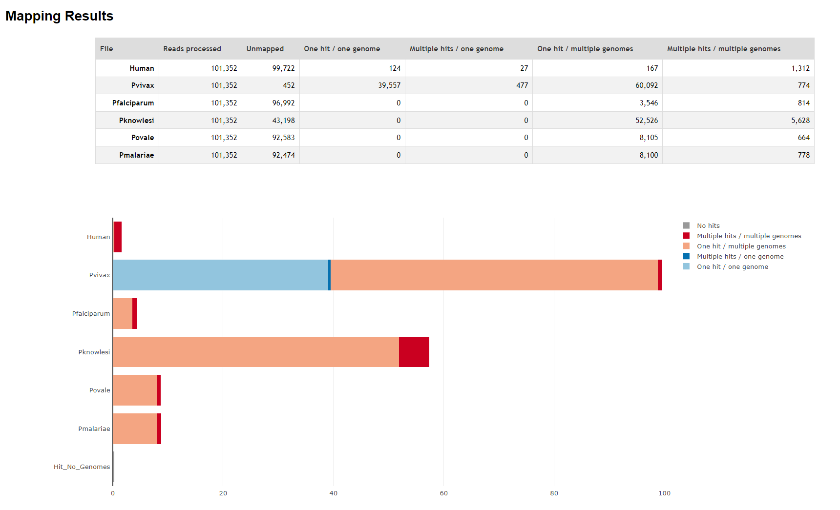
13.4 FastQ Screen

FastQ Screen is an utility that allows you to screen your FASTQ reads against a panel of genomes or known contaminants (like PhiX), to determine the origin of your sequences. In the case of malaria surveillance via AmpliSeq (or WGS), this allows us to screen for:

• mixed infections, common lab contaminants.
• human DNA contamination
• common lab contaminants
• artificial sequences (adapters, vectors)
• known problematic sequences (rRNA)

Under the hood, it uses a sequence aligner like bowtie or bwa (the latter of which we will use in the alignment or mapping chapter) to map the reads against various databases (= reference genomes or known contaminants). It also informs you where your reads map uniquely; both within and across species.

The full documentation for FastQ Screen can be found here.

Here is a short video introduction to the software:

Below we show an example of the output generated by FastQ Screen.

Example output of FastQ Screen for a P. vivax sample.

Exercises

• Download the Shiny app from Moodle, inspect the FastQC outputs and answer the questions.

13.5 Trimmining - trimmomatic

Note

There exist many alternative tools for trimming and filtering FASTQ files, such as fastp, Cutadapt and Trim Galore (which is a wrapper around Cutadapt and FastQC).

This tutorial focuses on fastqc + trimmomatic for historical reasons (being used in the ), but fastp is becoming more popular nowadays.

Trimmomatic is a tool that can:

• Trim low quality bases at the start and end of sequences
• Filter low quality reads (e.g., too short after trimming)
• Remove adapter sequences

Why do adapter sequences show up in reads?

Recall the structure of the library fragments shown in Figure 13.3, in particular the location of the adapters. The sequencing primer where sequencing commences is located downstream from the adapters and indices on the 5’ end. However, if the sequencing extends beyond the length of the DNA insert (i.e. the insert is shorter than the sequencing length), it enters into the adapter sequence on the opposite end of the fragment (on the 3’ end). These adapters need to be trimmed, but things are tricky because often times these are only incomplete partial adapter sequences.

More information can be found on page 5 of the Trimmomatic manual.

You can check the usage of trimmomatic by simply invoking the command without any arguments: trimmomatic

Usage:
    PE [-version] [-threads <threads>] [-phred33|-phred64] [-trimlog <trimLogFile>] [-summary <statsSummaryFile>] [-quiet] [-validatePairs] [-basein <inputBase> | <inputFile1> <inputFile2>] [-baseout <outputBase> | <outputFile1P> <outputFile1U> <outputFile2P> <outputFile2U>] <trimmer1>...
or:
    SE [-version] [-threads <threads>] [-phred33|-phred64] [-trimlog <trimLogFile>] [-summary <statsSummaryFile>] [-quiet] <inputFile> <outputFile> <trimmer1>...
or:
    -version

We can immediately see that there are two different versions, one for paired-end and one for single-end reads, as well as an option to specify the type of Q score (-phred33, which is not the default!).

Some of the other important options are trimmomatic:

Option	Meaning
inputFile1/2	The input fastq reads (.gz compression is allowed).
outputFile1/2P	Name of output file containing the paired reads from fastq pair 1/2.
outputFile1/2U	Name of output file containing the unpaired reads from read pair 1/2 (e.g., when its matching read was discarded).
ILLUMINACLIP:adapters.fa:2:30:10	Perform adapter removal. Requires a file containing known Illumina adapter sequences (like Nextera/TruSeq or specific to your protocol like for AmpliSeq).
SLIDINGWINDOW	Perform sliding window trimming, cutting once the average quality within the window falls below a threshold.
LEADING	Cut bases off at the start of a read, if the quality is below the threshold.
TRAILING	Cut bases off at the end of a read, if the quality is below the threshold.
MINLEN	remove reads that are too short

For the AmpliSeq pipelines, we generally stick to the following options:

• ILLUMINACLIP:adapters.fa:2:30:10: cut off Illumina specific adapters from the read (stored in adapters.fa).⁸
• LEADING:3: trim bases from the start of the read if they drop below a Q score of 3 (or N).
• TRAILING:3: trim bases from the end of the read if they drop below a Q score of 3 (or N).
• SLIDINGWINDOW:4:15: scan the read with a 4-base wide sliding window, cutting when the average quality per base drops below 15.
• MINLEN:36: remove reads that are shorter than 36 bases.

⁸ For AmpliSeq, an example can be found here. For generic WGS data, Trimmomatic comes with a few example files. On our workstations, they can be found in ${CONDA_PREFIX}/share/trimmomatic/adapters/NexteraPE-PE.fa

trimmomatic PE \
    -phred33 \
    -trimlog trimreport.txt \
    sample_R1_001.fastq.gz \
    sample_R2_001.fastq.gz \
    sample_R1_001.trim.fastq.gz \
    sample_R1_001.trim.unpaired.fastq.gz \
    sample_R2_001.trim.fastq.gz \
    sample_R2_001.trim.unpaired.fastq.gz \
    ILLUMINACLIP:adapters.fa:2:30:10 \
    LEADING:3 \
    TRAILING:3 \
    SLIDINGWINDOW:4:15 \
    MINLEN:36

For more detailed info on all these commands, check out the trimmomatic manuaul.

Tip

The threads option allows you to process multiple samples simultaneously to speed up the analysis. We will see more on parallelization and multi-threading later. In your CodeSpace environment, you can choose 2 or 4 threads, depending on the number of cores you selected.

Exercises

• Try trimming a single pair(!) of reads.
• Run FastQC again on the trimmed reads and compare the results with the original FastQC report.
• Write a script to trim multiple reads in one go and use it to analyse all the paired read in the Peruvian P. falciparum AmpliSeq dataset. Remember that you can use pseudo-code to start out with.
  • Afterwards, compare your approach to the trim.sh script in the ./training/scripts directory.
• Can you guess what the following line does? base=$(basename ${read_1} _1.fastq.gz)
  • Hint: $(command) is a way to run a command inside another command or statement, so try figuring out what the command between the brackets does first.

Bonus exercise: trim all the read files for the Vietnam P. vivax WGS data too and compare the FastQC differences.

Tip 13.2: Looping over paired FASTQ files in bash

When writing scripts that iterate over paired FASTQ files, you can use the concepts that we introduced in Tip 8.1.

A minimal example is provided below:

#!/usr/bin/env bash

# loop through the first read of each pair
for read_1 in ../data/fastq/*_R1_001.fastq.gz

do

    # extract the sample name and print it
    sample_name=$(basename "${read_1}" _R1_001.fastq.gz)

    echo "Read 1 = ${sample_name}_R1_001.fastq.gz"
    echo "Read 2 = ${sample_name}_R2_001.fastq.gz"

done

Tip 13.3: Evaluating many reports at once: MultiQC

As a bonus exercise, have a look at MultiQC. This is a tool that allows you to aggregate the output results from many different samples into a single report. It supports many different bioinformatics tools, including FastQC.

You can install it on your own environment using the following command: conda install multiqc and play around with it.

---

Additional resources

• Sequencing library construction, adapters and indexing:

  • https://teichlab.github.io/scg_lib_structs/methods_html/Illumina.html
  • https://www.umassmed.edu/contentassets/5ea3699998c442bb8c9b1a3cf95dbb24/indexing-and-barcoding-for-illumina-nextgen-sequencing.pdf
  • https://www.lubio.ch/blog/ngs-adapters
  • https://www.umassmed.edu/globalassets/deep-sequencing-core/indexing-and-barcoding-for-illumina-nextgen-sequencing-2021.pdf
  • https://knowledge.illumina.com/library-preparation/general/library-preparation-general-reference_material-list/000003275
  • https://support.illumina.com/ko-kr/bulletins/2020/12/how-short-inserts-affect-sequencing-performance.html
  • https://support-docs.illumina.com/SHARE/IndexedSeq/indexed-sequencing.pdf

• Demultiplexing:
  • https://s3-us-west-2.amazonaws.com/oww-files-public/a/a5/IlluminaParsing_v1-2.pdf
• Paired-end sequencing:
  • https://www.illumina.com/science/technology/next-generation-sequencing/plan-experiments/paired-end-vs-single-read.html
  • Orientation of (index) reads: https://seekdeep.brown.edu/illumina_paired_info.html

Library preparation and bridge amplification on flow cell. Sequencing-by-synthesis and fluorophore imaging or base calling. Figure 13.2: Paired-end sequencing and alignment. (Source: Illumina 2017) Figure 13.3: Construction of a sequencing library fragment through adapter ligation: P5 (red) / P7 (green) = sequences for anchoring to flow cell; (Rd1 SP (orange) / Rd2 SP (blue) = read 1/2 sequencing primer; index/barcode 1/2 = sample identifiers for multiplexing (Source: Illumina 2020). Fluorescent signals from clusters on flow cell (Source: Illumina 2016). Figure 13.4: FASTQ quality scoring and ASCII offsets. (Source: Batut et al.; Hiltemann et al. 2023) Figure 13.5: ASCII table Example output of FastQC. Note the decreasing scores towards the end of the read. Example output of FastQ Screen for a P. vivax sample.

Batut, Bérénice, Maria Doyle, Alexandre Cormier, Anthony Bretaudeau, Laura Leroi, Erwan Corre, Stéphanie Robin, gallantries, and Cameron Hyde. “Quality Control (Galaxy Training Materials).” https://training.galaxyproject.org/training-material/topics/sequence-analysis/tutorials/quality-control/tutorial.html.

ClevaLab. 2022a. “A Step-by-Step Guide to NGS.” https://www.clevalab.com/post/a-step-by-step-guide-to-ngs.

———. 2022b. “Next Generation Sequencing - a Step-by-Step Guide to DNA Sequencing.” YouTube. https://www.youtube.com/watch?v=WKAUtJQ69n8.

Hiltemann, Saskia, Helena Rasche, Simon Gladman, Hans-Rudolf Hotz, Delphine Larivière, Daniel Blankenberg, Pratik D. Jagtap, et al. 2023. “Galaxy Training: A Powerful Framework for Teaching!” Edited by Francis Ouellette. PLoS Comput Biol Computational Biology 19 (1): e1010752. https://doi.org/10.1371/journal.pcbi.1010752.

Illumina. 2008. “Multiplexed Sequencing with the Illumina Genome Analyzer System.” https://www.illumina.com/documents/products/datasheets/datasheet_sequencing_multiplex.pdf.

———. 2016. “Overview of Illumina Sequencing by Synthesis Workflow.” YouTube. https://www.youtube.com/watch?v=fCd6B5HRaZ8.

———. 2017. “An Introduction to Next-Generation Sequencing Technology.” https://www.illumina.com/content/dam/illumina-marketing/documents/products/illumina_sequencing_introduction.pdf.

———. 2020. “How Short Inserts Affect Sequencing Performance.” https://support.illumina.com/ko-kr/bulletins/2020/12/how-short-inserts-affect-sequencing-performance.html.

———. 2021a. “Learn about Illumina’s Next-Generation Sequencing Workflow.” YouTube. https://www.youtube.com/watch?v=oIJaA6h2bFM.

———. 2021b. “Indexed Sequencing on Illumina Systems.” https://support-docs.illumina.com/SHARE/IndexedSeq/indexed-sequencing.pdf.

———. n.d. “Next-Generation Sequencing Glossary.” NGS Terminology. https://www.illumina.com/science/technology/next-generation-sequencing/beginners/glossary.html.

Launen, Loren. 2017. “Illumina Sequencing (for Dummies).” https://kscbioinformatics.wordpress.com/2017/02/13/illumina-sequencing-for-dummies-samples-are-sequenced/.

Ledergerber, C., and C. Dessimoz. 2011. “Base-Calling for Next-Generation Sequencing Platforms.” Briefings in Bioinformatics 12 (5): 489–97. https://doi.org/10.1093/bib/bbq077.

Piper, Mary E., Meeta Mistry, Jihe Liu, William J. Gammerdinger, and Radhika S. Khetani. 2022. “Hbctraining/Intro-to-Rnaseq-Hpc-Salmon-Flipped: Introduction to RNA-Seq Using Salmon Lessons from HCBC (First Release),” January. https://doi.org/10.5281/ZENODO.5833880.

Rodriguez, Raphaël, and Yamuna Krishnan. 2023. “The Chemistry of Next-Generation Sequencing.” Nature Biotechnology 41 (12): 1709–15. https://doi.org/10.1038/s41587-023-01986-3.

Shendure, Jay, Shankar Balasubramanian, George M. Church, Walter Gilbert, Jane Rogers, Jeffery A. Schloss, and Robert H. Waterston. 2017. “DNA Sequencing at 40: Past, Present and Future.” Nature 550 (7676): 345–53. https://doi.org/10.1038/nature24286.

University of Exeter DNA sequencing service. “Introduction to Genomics.” https://biomedicalhub.github.io/genomics/01-part1-introduction.html.